Chapter 4 — Auxiliary Windows
Alongside the main window (3D viewport plus Inspector), RadianceKit manages six additional windows, all of which are opened via the Help menu. The menu has eight entries, from top to bottom: User Guide (⌘?), Keyboard Shortcuts (⌘/), Open Training Logs… (⇧⌘L), Open Exports Folder…, Manage Storage…, Pareto Dashboard… (⇧⌘D), Holdout Analysis… (⇧⌘H), BayesOpt Console… (⇧⌘B). The two "Open …" entries don't open an app window but the Finder; for this reason they aren't covered further here. Three of the windows — Dashboard, Holdout, BayesOpt — are standalone analysis tools: they operate independently of the main window and read or write JSON files on disk. You open each of these three windows via the Help menu, and then choose for yourself which file or folder you want to evaluate — via "Open Reports Folder…", "Open transforms.json…", or the "Start" button. These three windows are the only ones that aren't localised: their buttons, sliders, and column headers appear in English in every language version. So the labels mentioned here are exactly what you'll see on screen.
The three simple windows (User Guide, Keyboard Shortcuts, Manage Storage) and the two folder menu items (Open Training Logs / Open Exports Folder) each get a short entry per control. The three analysis windows are documented in more detail — each with an introduction explaining what you see in the window, when you should open it, and how to interpret the displayed picture.
At the end of the chapter there's a cross-reference section to the Inspector of the main window: what you can meaningfully read off the live loss chart and the Gaussian count display while a training run is in progress.
User Guide (W1–W4)
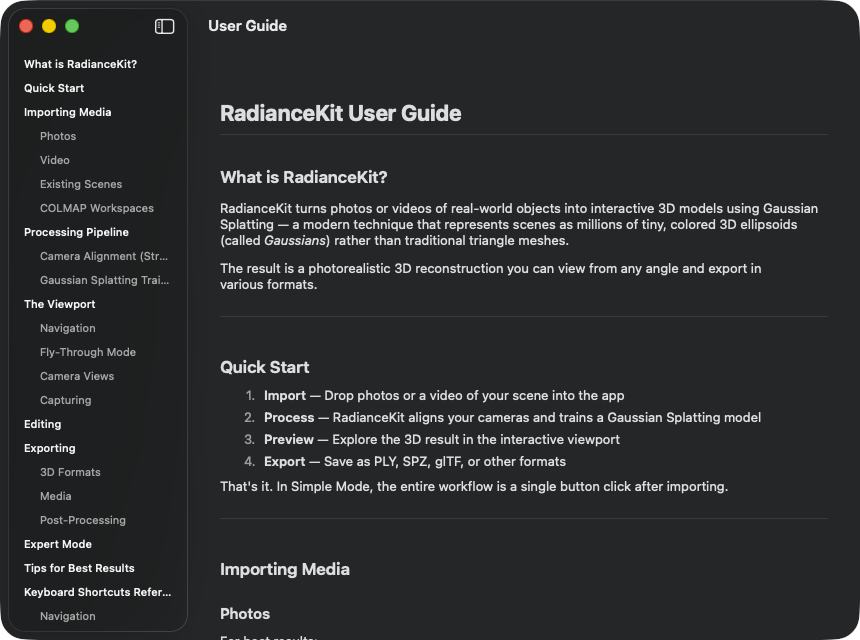
What it is: A built-in help window that renders the guide_<language>.md shipped with the app. The language is derived from Settings (General tab → Language) or, if that's set to "System", from the macOS language preferences. The layout is classic: a sidebar with all headings on the left, the body text on the right.
When you need a quick reminder about a single point — i.e. as a substitute for keywords. This manual is the detailed reference; the built-in help window is the short version for quick lookup. It gets updated with every app release, but is kept more superficial in content.
W1NavigationSplitView (Sidebar + Detail)
WHERE
Help → User Guide (⌘?).
TECHNICAL
Two-column layout with a narrow sidebar (at least 180 pt wide) for the content tree and a scrollable detail area for the actual Markdown content. The window has a minimum size of 700 × 500 pt. When first opened, the window loads the matching guide_<lang>.md from the app bundle (fallback guide_en.md), parses it into block records (headings H1–H4, paragraphs, lists, tables, dividers), and separately extracts the heading structure for the sidebar. Inline formatting (bold, italic, code span) is rendered via the built-in Markdown engine. The language is read from the app settings, with the special case of Chinese (zh-Hans) and Brazilian Portuguese (pt-BR), which are kept as full locale tags because these variants differ from plain zh and pt, respectively.
W2List (heading sidebar)
WHERE
Left column in the User Guide window.
TECHNICAL
List of all H2 and H3 headings in the current Markdown document. H2 entries appear without indentation with medium font weight, H3 entries with 16 pt left indentation and reduced foreground style. All other levels — H1 as well as H4 and deeper — do not appear in the sidebar, because they would otherwise make it cluttered. Anchor IDs are generated from the heading text via slugification (lowercase + spaces to dashes + filtering to letters/numbers/dashes — the same algorithm GitHub uses for its Markdown anchors, so external URLs to the docs could potentially land on the same anchor). The list uses the native macOS style.
W3Button (heading → anchor jump)
WHERE
One button per sidebar row.
TECHNICAL
Each sidebar entry is a button that sets the current anchor, but visually looks like a list entry. An observer variable then triggers the scroll jump to the corresponding anchor with a smooth animation over 0.3 s. After the jump, the anchor value is reset so that the next click on the same anchor fires again (otherwise the observer wouldn't trigger again, because the value hasn't changed).
W4ScrollView (detail content)
WHERE
Right column.
TECHNICAL
Scrollable, vertically stacking content area with lazy rendering, because longer guides can easily have more than 200 Markdown blocks — a non-lazy variant would instantiate all of them at once. Each block gets its own ID, either the heading anchor (which every heading gets, regardless of level) or an index placeholder. Maximum width is 720 pt, padding 32 horizontal / 24 vertical, so that long lines keep a well-readable layout. Tables are rendered cell by cell with horizontal stacks and divider lines; inline code by the built-in Markdown engine. Actual code blocks are currently treated as paragraphs — a known limitation of the help window.
Keyboard Shortcuts (W5–W6)
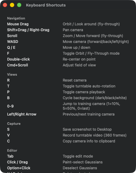
A static reference list in five sections. Navigation: Mouse Drag (Orbit/Fly), Shift+Drag/Right-Drag (Pan), Scroll (Zoom), WASD (Fly-Through movement), Q/E (Up/Down), F (Toggle Orbit/Fly), Double-click (Re-center), Cmd+Scroll (FoV adjust). Views: R (Reset Camera), T (Auto-Rotation), P (Camera Playback), B (Background cycle), 0–9 (Jump to Training Cam 1=10%/5=50%/0=last), Left/Right Arrow (Prev/Next Cam). Capture: S (Screenshot to Desktop), V (Turntable video), C (Copy Camera Info). Editor: Tab (Edit mode), Click/Drag (Paint-Select), Option+Click (Deselect), X / Delete (Delete selection), Cmd-Z (Undo last deletion), [ / ] (Decrease/increase brush size), Esc (Clear selection). Training: Option+Space (Pause/resume training), Cmd+E (Export scene). That's all that's here — Start, Cancel and the extensions are reached via the Training menu (Chapter 1).
What it is: A simple static overview of all keyboard shortcuts — Navigation, Views, Capture, Editor, Training. The content is hard-coded and isn't loaded from a file.
When you're looking for the fastest way to do something in the viewport. WASD fly-through, R for camera reset, B for background cycling — they're all here.
W5ScrollView (content area)
WHERE
Help → Keyboard Shortcuts (⌘/).
TECHNICAL
A simple scroll area with a vertical list inside. Padding 20 all around, no sidebar navigation tree (the list is short enough). Content is grouped into five sections (Navigation, Views, Capture, Editor, Training). One row per key combination with translatable text in both columns. Left column (key code) fixed at 180 pt width, so the descriptions on the right stay vertically aligned. No interaction other than scrolling — clicking a row doesn't trigger anything, the keyboard shortcuts are real keyboard modifiers in the menu and on the viewport.
W6VStack (shortcut sections)
WHERE
Inside the ScrollView.
TECHNICAL
Left-aligned stacked sections with 16 pt spacing. Within each of the five sections: a heading followed by a sequence of rows. Headings use a secondary subheadline style — deliberately not a title format, because the sections don't need to be navigable. Content is deliberately flat (no disclosure, no search, no filter), so the component runs unchanged on every macOS version and the file stays readable.
Manage Storage (W7–W12)
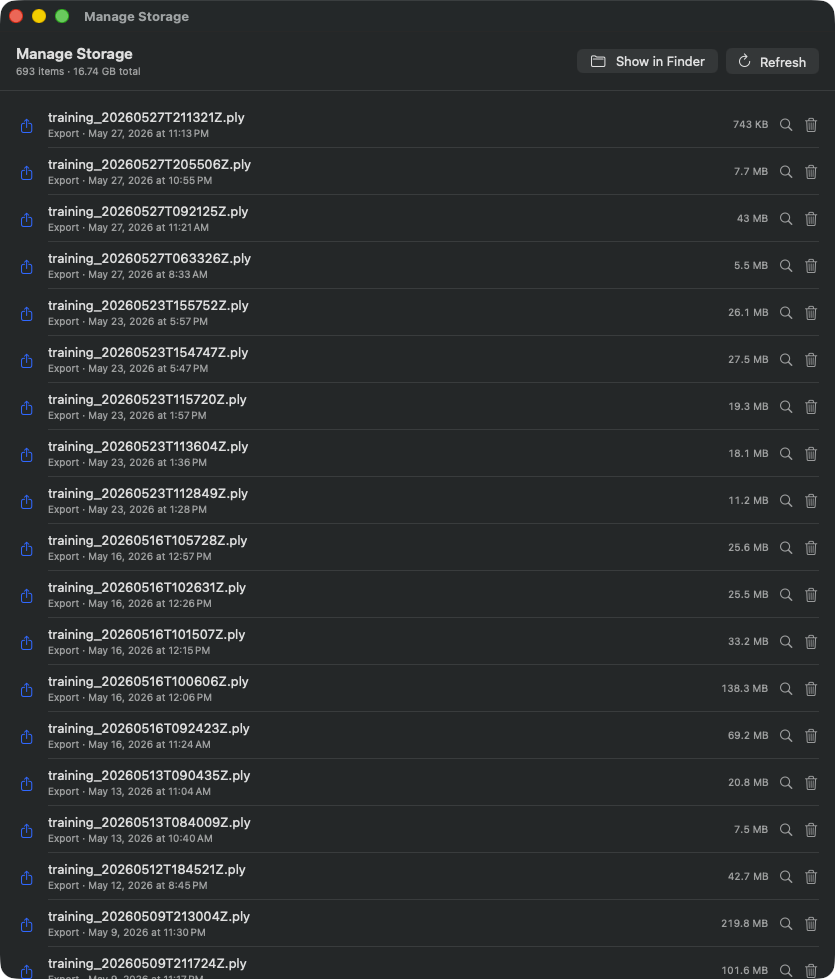
Table view of all files managed by RadianceKit. Header counts 1,356 items, 55.1 GB total size. Toolbar at top: "Show in Finder" + "Refresh". Each row: export icon, filename (e.g. training_20260718T194416Z.ply), export date, size (varies here from 7.8 MB to 2.24 GB), magnifying-glass icon (Reveal), and trash-can icon (Move to Trash). Sorting is first by category and within a category by date, newest at the top. In this screenshot PLY exports dominate, because this location was mainly used to back up training results.
What it is: A disk-usage overview for everything RadianceKit stores under ~/Documents/RadianceKit/ — logs, exports, scenes, capture bundles (from the iOS companion), imports (staging copies of the input images). Each entry has a size in bytes and two buttons: "Show in Finder" and "Move to Trash". This is NOT automatic cleanup — the app doesn't delete anything on its own; you decide per entry. This window is localised: in German it's called "Speicher verwalten", the two header buttons are called "Im Finder anzeigen" and "Aktualisieren", the row buttons "Im Finder anzeigen" and "In den Papierkorb legen". The English names in the entries below are the labels from the English version.
When your disk fills up. The logs in particular accumulate (one JSONL per training attempt, plus the _qualityMetrics.json); the exports of course too (PLY is 100% raw data, one per export). Also useful after a crash, when the imports staging directory still has old copies of the input images lying around.
W7Button "Show in Finder"
WHERE
Header at the top right of the storage browser window.
TECHNICAL
Opens the RadianceKit data folder in the Finder — exactly the directory whose contents this window lists. This lets you see the folder structure (Logs, Exports, Scenes, Captures, Imports) directly and also move or copy files using Finder itself. The action opens a new Finder window; the list in the window does not update as a result — that's what "Refresh" (W8) is for.
W8Button "Refresh"
WHERE
Header, next to the Finder button.
TECHNICAL
Triggers a background scan that runs on a user-initiated asynchronous task, so scanning large directory trees doesn't block the UI. The actual walk goes through every known subfolder (Logs, Exports, Scenes, Captures, Imports) and creates a storage entry for each direct child. For each entry the recursive size is determined — preferring the actual disk usage (including APFS hard-link sharing) with a fallback to the logical file size.
W9List (storage entries)
WHERE
Main content below the header.
TECHNICAL
List with this layout per row: category- specific SF Symbol icon (document for logs, upload arrow for exports, cube for scenes, iPhone for capture bundles, tray for imports), name + subtitle (kind label + formatted modification date), byte counter on the right (right-aligned, monospaced), Reveal button (magnifying-glass symbol), Trash button (trash can). Sorting: primarily by kind (scenes first, then exports, logs, captures, imports, other), secondarily by modification date descending (newest at top). While the scan is still running, a "Scanning…" progress indicator is shown instead. If nothing was found, an empty-state display with a tray icon appears.
W10Row button "Reveal in Finder"
WHERE
Per row, magnifying-glass symbol on the right.
TECHNICAL
Opens the Finder and selects the specific item (file or folder). Difference from W7: W7 opens the root directory; W10 selects exactly this one entry. Handy workflow: identify a large entry, click the magnifying glass, then copy it to, say, an external volume.
W11Row button "Move to Trash"
WHERE
Per row, trash icon to the right of the magnifying glass.
TECHNICAL
Triggers the confirmation dialog box (W12). Only after confirmation does the standard macOS "move to trash" operation run (i.e. reversible, not a direct delete). After successfully moving to trash, the entry is removed from the list and the total byte counter updates. On errors, a modal error dialog is shown.
W12ConfirmationDialog (delete confirmation)
WHERE
Triggered by W11, presented as a macOS sheet.
TECHNICAL
Standard confirmation dialog with a dynamic title "Delete <name>?" and a message line that explicitly points out that the entry will end up in the trash and can be restored from there (until the trash is emptied). Two buttons: "Move to Trash" as a destructive action (shown in red) and "Cancel" with an automatic Esc binding. The dialog is non-modal in the sense that it only blocks this window, not the whole app — that's the macOS standard for reversible deletions.
Pareto Dashboard (W13–W22)
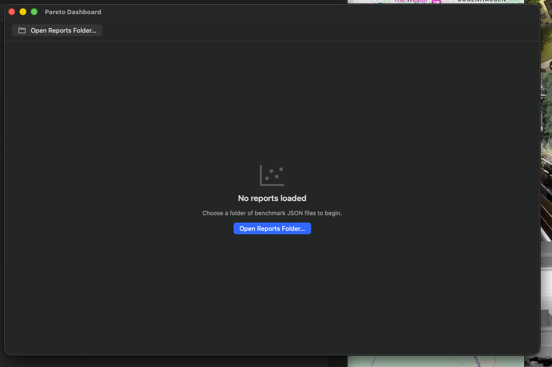
Empty state (right after first opening) — empty state with call-to-action „Open Reports Folder…". The data points appear as soon as training reports are loaded, see next shot.
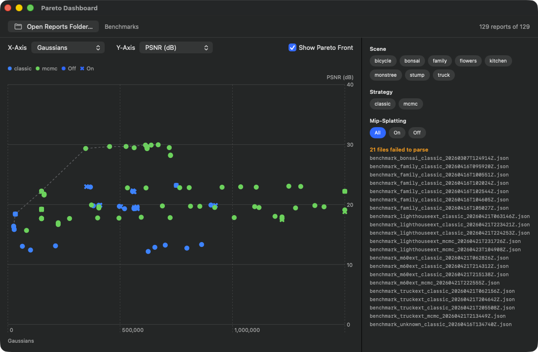
The header toolbar shows „384 reports of 384" on the right (all reports in the selected folder parsed successfully); to the left of the „Open Reports Folder…" button is the name of the loaded folder, here „Benchmarks". Axes: X-Axis picker set to Gaussians, Y-Axis picker set to PSNR (dB), next to it the active „Show Pareto Front" checkbox. Legend top left: blue = mcmc, green = classic, orange = hybrid, plus the symbol shape for Mip-Splatting On/Off. The dashed Pareto-front line runs along the best-achieved PSNR values and plateaus around PSNR≈30 dB from about 300K Gaussians onward; the point cloud extends beyond 1.5 million Gaussians. Filter chips on the right: over 30 scenes (including bicycle, bonsai, family, flowers, garden, kitchen, stump, truck, as well as the numbered 360, drone, and photo test series), 3 strategies (classic, hybrid, mcmc), 3 Mip-Splatting options (All, On, Off) with „All" active. No scene or strategy filter is currently set, hence the dense point cluster.
What it is: A multi-run comparison tool. You've trained several scenes in the past, or the same scene with different presets — a benchmark evaluation produces a JSON report file for each training run, containing among other things final PSNR, SSIM, LPIPS, Gaussian count, and wall-clock time. There is no toggle for this evaluation in the interface; the dashboard evaluates whatever is already present as a report in the selected folder. It reads an entire folder of such reports at once and plots them as a 2D scatter plot with selectable axes. In addition, the Pareto front (the set of non-dominated points) is drawn as a dashed line.
After you've created at least three or four training reports. With fewer points, the frontier line isn't meaningful. Typical use case: you tried to reconstruct an outdoor scene, and ran P3 Balanced (Classic), P4 Quality (Classic), P8 Quality (MCMC), and P9 Drone / Aerial one after another — now you want to know which configuration delivers the best PSNR per second of training time, or which needs the fewest Gaussians for a given PSNR.
Both axes are freely selectable (X axis: Gaussians, training time, PSNR, SSIM, LPIPS, …; Y axis likewise). The Pareto-front calculation knows for each metric whether „smaller = better" (LPIPS, Gaussians, Training Time, BRISQUE) or „bigger = better" (PSNR, SSIM, FSIM, MS-SSIM) — so the line runs, depending on the chosen axes, from bottom left to top right or from top left to bottom right, always along the best-achieved combination. A point is Pareto-optimal if NO other point is at least as good in BOTH dimensions (i.e. no other point dominates it). Pareto-optimal points lie on the line, other points to the right/above (depending on axis orientation) of it. Points ON the line are the real candidates for „best preset"; points FAR from the line represent wasted training time.
You can restrict the selection to a specific scene (e.g. if you only want to compare outdoor runs), to a specific strategy (classic, hybrid, or mcmc), or to Mip-Splatting on/off (Mip-Splatting is an optional advanced setting, which is why the direct comparison is worthwhile).
You have three reports for the „truck" scene in one reports folder: Run A (P4 Quality (Classic), 524K Gs, 105 s, PSNR 23.4), Run B (P8 Quality (MCMC), 150K Gs, 693 s, PSNR 24.6), Run C (P5 Ultra Detail, 1.25M Gs, 312 s, PSNR 25.8). Set the X axis to Training Time, the Y axis to PSNR. Run B is top right, Run C even further top right, Run A bottom left. The Pareto front connects A and C — both non-dominated. Run B is „lost" (C is better in both time AND PSNR). Insight: for „truck", the MCMC route isn't worthwhile; either fast+ok (A) or long+very good (C). Save the configuration from C as its own preset (Inspector → I1 Save Preset).
Next action: Save the best configuration as a preset. Specifically: look at the Pareto points (hovering shows PSNR/SSIM/LPIPS/Gs/Time in the tooltip), decide which one best fits your time-vs-quality trade-off, open the corresponding report (filename contains the run timestamp), copy its training configuration into a new run, or save it as a preset via the Inspector after your next training session.
W13„Open Reports Folder…" button
WHERE
Toolbar, top left.
TECHNICAL
Opens a folder-selection dialog with the prompt „Select a folder containing benchmark .json reports". After confirmation, a background task runs that parses all .json files in the folder sequentially. Faulty reports (broken JSON, wrong schema) are collected and shown at the bottom of the sidebar as „N file failed to parse" — no crash. If a second click happens while a first load is still running, the previous task gets cancelled, so that two results don't write to the state simultaneously.
The selected folder isn't remembered permanently: after opening the window via Help → Pareto Dashboard… (⇧⌘D) you select it again here. The name of the loaded folder then appears to the right of the button.
W14„X-Axis" picker
WHERE
Above the chart, on the left.
TECHNICAL
Menu picker with all available metric axes of the dashboard module (PSNR, SSIM, LPIPS, Gaussian count, training time, and so on). Default is Gaussian count. When switching, the hovered point is reset, because a previously highlighted position in the old axis coordinate system no longer makes sense after an axis change. The picker's width is limited to its content, so it doesn't stretch across the entire width.
W15„Y-Axis" picker
WHERE
Above the chart, next to X-Axis.
TECHNICAL
Identical to W14, except the default is PSNR. The axis selection is stored independently, so the user can also choose nonsensical combinations (X=PSNR, Y=PSNR — would throw all points onto a diagonal). Such combinations aren't blocked, though; this is a deliberate decision, because a comparison of „SSIM vs PSNR" can indeed be interesting, to see how consistently the metrics behave.
W16„Show Pareto Front" toggle
WHERE
Next to the axis pickers, on the right.
TECHNICAL
A checkbox, checked by default. The Pareto front is overlaid on the point cloud as a line on the chart — dashed (dash pattern 4–4), gray semi-transparent, line width 1.5 pt. Note: In the shipped version, the checkbox has no effect on the chart — the front line is always drawn, whether checked or not. The front is recalculated on every axis change and after every filter change.
W17„Scene" filter chips
WHERE
Right sidebar in the dashboard window.
TECHNICAL
Filter chips for every scene that appears in the loaded reports. A custom flow layout automatically wraps chips into multiple lines once the width is exhausted. Active chips get the accent background, inactive ones a neutral standard material background. Multi-selection is possible (set semantics); if no chip is selected, all scenes are considered „passed through" — i.e. the set logic is „empty selection = everything", not „empty selection = nothing".
W18„Strategy" filter chips
WHERE
Below the Scene filter in the sidebar.
TECHNICAL
Just like W17, but for training strategies — typically the three values „classic", „hybrid" and „mcmc", derived from the strategy field in the benchmark report JSONs. Helpful if you've mixed reports from multiple strategies and only want to see one kind (e.g. „only show MCMC runs, because I've already excluded Classic").
W19„Mip-Splatting" filter chips
WHERE
Below the Strategy filter in the sidebar.
TECHNICAL
A three-valued filter (instead of a set like W17/W18): „All" / „On" / „Off". Background: Mip-Splatting is a multi-scale extension that helps or doesn't depending on the scene — which is why it remains a deliberately toggleable setting rather than a default. If you're doing Mip on/off comparisons, you often want to separate them very sharply. Hence the dedicated ternary filter with the states „pass everything through", „only Mip on", „only Mip off". The sidebar section appears as soon as the loaded set contains any reports at all — so practically always; it only disappears when nothing at all is loaded.
W20ChipButton (filter toggle, all/on/off)
WHERE
Helper component, used in W17/W18/W19.
TECHNICAL
A minimalist button wrapper. Content: label text with caption font size and padding of 10 horizontal / 5 vertical. Background conditional: if active → app accent color with white text; otherwise a neutral standard material background with the normal text color (adapts to light and dark appearance). Shape is a capsule (pill-shaped). Plain button style, so the capsule material isn't overlaid by a system border.
W21Chart (Pareto scatter)
WHERE
Center area of the dashboard.
TECHNICAL
Swift Charts diagram with two layers: 1. a point per report — position from the selected X and Y metrics, color by strategy, symbol by Mip status. Symbol size normally 80, highlighted 200 (when the ID matches the currently hovered report). 2. a line for the Pareto front (see W16 — it's always drawn). Additionally, the currently hovered point displays the scene name as a small capsule above it.
Chart overlay: a transparent rectangle registers mouse movement; each frame, the Euclidean nearest point position in the plot frame is determined and the hovered report is updated if the distance is under 24 px (otherwise reset). This gives you the tooltip without clicking — hovering is enough.
W22Tooltip (hover detail)
WHERE
Below the chart, shown on hover.
TECHNICAL
Horizontal stack: scene name (headline), strategy tag (caption), divider line, then PSNR/SSIM/LPIPS/Gs/Time metrics each in its own small vertical group (label + monospaced value). If Mip was enabled, an additional „Mip" capsule tag in accent color. Background is a semi-transparent blur, rounded rectangle with an 8 pt radius. Only shown when the mouse is actually over a point. Disappears automatically when the mouse leaves.
Holdout Analysis (W23–W29)
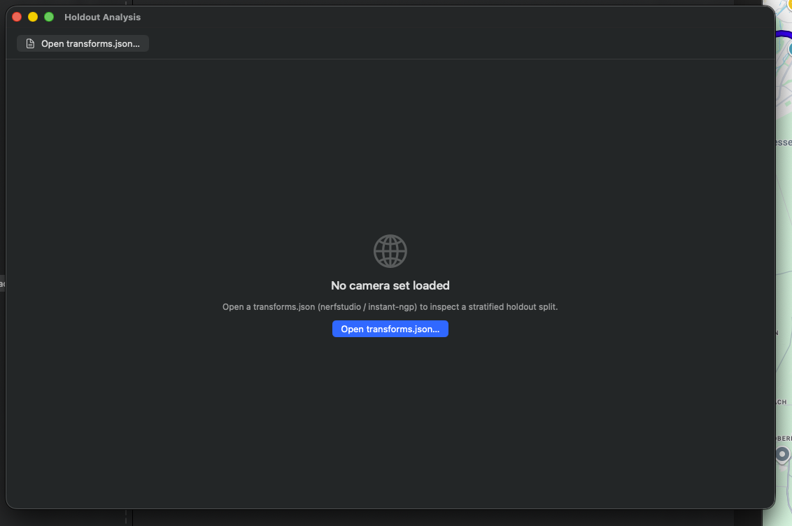
Empty state with an empty-state placeholder and call-to-action "Open transforms.json…". Accepts NeRF-Studio and Instant-NGP format. The camera markers appear as soon as a transforms.json is loaded — see the next figure.
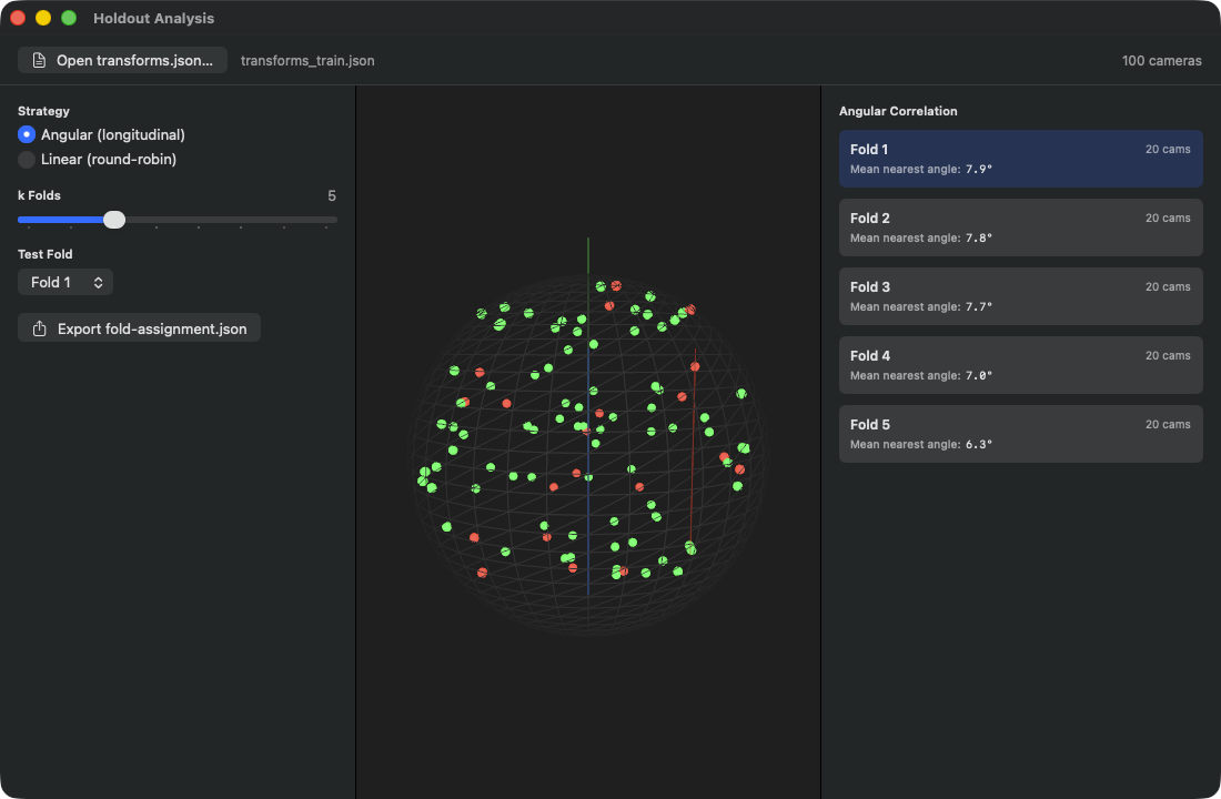
Header shows the loaded file (transforms.json) and cam count ("86 cameras"). Left sidebar: strategy picker with two options — Angular (longitudinal) active (sorts the cameras by their longitudinal angle around the orbit and then distributes them round-robin across the folds) vs Linear (round-robin) (the same round-robin distribution, but by image order instead of by viewing angle). The k-folds slider is set to 5, the test-fold picker to Fold 1. The export button generates a fold-assignment.json for further use in external evaluation tools. Middle panel: 3D globe projection of all 86 cameras, distributed over the whole sphere — green dots = train, red dots = current test fold (Fold 1 with 18 cameras). Right sidebar (Angular Correlation): per fold the camera count + mean nearest angle (Fold 1: 18 cams / 8.5°, Fold 2: 17 / 6.1°, Fold 3: 17 / 6.2°, Fold 4: 17 / 6.7°, Fold 5: 17 / 6.4°) — a smaller value means that each test camera has a nearby training camera, so the test is easier.
What it is: A 3D visualizer for your camera arrangement with cross-validation logic. You load a transforms.json (the standard format used by Nerfstudio / Instant-NGP for camera poses), the app reads all cameras, projects their viewing directions onto a unit sphere, and shows them as small sphere markers on a virtual globe. It then splits the cameras into k folds (using the chosen strategy: angular or linear), marks the training portion green and the test portion (holdout) red, and calculates an angular-correlation score per fold that tells you how far the test fold is from the training fold in viewing-angle space.
When you want to do holdout evaluation — in other words: how well does your model generalize to unseen viewing angles? The default during training is "every-8th view as holdout" (Mip-NeRF360 convention), but that's a very linear split. If your images are, for example, clustered temporally (one side of the object first, then the other), then "every-8th" isn't representative — a random sequence position ends up in the test set, but all its neighbors are in the training set, which is too easy. With "angular" you instead stratify across viewing-angle space: each fold contains cameras from all areas of the orbit, so the test genuinely probes generalization gaps.
Angular vs Linear: - Angular (default): sorts all cameras by their longitudinal angle (φ coordinate around the Y axis) and then distributes them round-robin across the k folds — the first camera in the ring goes into Fold 1, the second into Fold 2, and after k cameras the cycle starts over. Advantage: every fold contains cameras from all directions of the orbit, evenly distributed around the ring. Good for classic orbit captures, because the split no longer depends on the capture order. - Linear (round-robin): the same round-robin distribution, but over image position instead of angle (fold index = image_index modulo k). This is the simple "every-k-th" split. Works well if the image order has NO spatial bias (e.g. randomly ordered drone footage). Works poorly if the images cluster temporally — then neighboring frames end up in different folds and the test becomes too easy.
In the 3D globe you can see immediately: green dots (training) and red dots (test). If the red dots all cluster in one corner, the holdout is poor (not a good generalization test). If they're evenly distributed among the green ones, it's good. The angular-correlation score per fold (right sidebar, in degrees) additionally tells you: a smaller value = the test is close to the training set (every test camera has a nearby training camera, easier test); a larger value = the test is far from the training set (harder generalization).
You captured your truck scene with 251 images, exported a nerfstudio file via menu item M33 (Export SfM transforms.json). Open the Holdout window (⇧⌘H), load the JSON via "Open transforms.json…", look at the globe. k=5 (default) gives you 5 folds. Click "Fold 3" — see if the red markers are reasonably even. If so: "Export fold-assignment.json". The exported file is meant for external evaluation tools (Nerfstudio, Instant-NGP); RadianceKit itself doesn't read it back in and continues training against its own holdout standard "every-8th". So the window's purpose here is to help you judge whether your camera set even allows for a fair test.
W23Button "Open transforms.json…"
WHERE
Toolbar, top left.
TECHNICAL
Opens a file-selection dialog restricted to JSON files. Once confirmed, the holdout module loads the file. The loader parses both the nerfstudio format (camera intrinsics plus a list of frames with image path and transform matrix) and the instant-ngp format (same structure). Per frame, the viewing direction is extracted from the transform matrix (z-axis of the camera's local basis) and stored. If parsing fails, a message appears in the left sidebar — but only if a scene had already been loaded there; on the very first attempt the window stays in the empty state without a visible message.
The loaded file is not remembered permanently: after reopening the window via Help → Holdout Analysis… (⇧⌘H) you select it again here. Its name then appears to the right of the button.
W24Picker "Strategy" (angular/linear)
WHERE
Left sidebar, top.
TECHNICAL
Radio picker with two options: Angular and Linear. Switching the strategy automatically triggers a recomputation of the folds. The viewing directions are a list of 3D unit vectors on the sphere; the angular strategy sorts them by their longitudinal angle φ and then assigns them round-robin to the folds, while the linear strategy makes the same round-robin assignment based on the frame index and ignores the geometry entirely. Both strategies therefore produce equally sized folds; they only differ in what they sort by beforehand.
W25Slider "k Folds"
WHERE
Left sidebar, middle.
TECHNICAL
Slider from 3 to 10, step size 1. When changed, the fold computation is automatically re-triggered, so the fold list, training/test indices, and per-fold score are immediately recalculated. The chosen value is displayed as monospaced-digit text to the right of the label.
Rule of thumb: k=5 is the default (gives you 20% test per fold, which is common for cross-validation). k=10 if you have a lot of data and need more folds for statistical power. k=3 if you have little data.
W26Picker "Test Fold"
WHERE
Left sidebar, below the k slider.
TECHNICAL
Menu picker. It lists exactly as many entries as folds are set, labeled "Fold 1" through "Fold N". If the previously selected index is ≥ k (e.g. because you reduced k from 10 to 5), it is automatically reset to 0. The chosen test fold is shown red on the globe, all others green.
W27Button "Export fold-assignment.json"
WHERE
Left sidebar, bottom.
TECHNICAL
Opens a save dialog with the default file name fold-assignment.json. Once confirmed, the holdout module encodes the current split into a JSON schema (per-frame fold assignment plus a strategy metadata block). The file is meant for external evaluation tools — RadianceKit does not read it back in. The button is grayed out as long as no camera file is loaded. Success is reported as "Saved to (filename)", a write error as "Export failed: …" — both appear in the same place below the button and both in green text, so the color doesn't distinguish the cases.
W28SCNView (3D Camera Globe)
WHERE
Middle panel of the Holdout window.
TECHNICAL
SceneKit globe view. The scene consists of: a wireframe sphere (radius 1.0, 36 segments, dark gray), three colored axis stubs (red/green/blue for X/Y/Z, each 1.2 long), and per camera a small marker sphere (radius 0.03) at the corresponding viewing-direction position on the unit sphere (slightly offset outward so it doesn't disappear INSIDE the wireframe sphere). The markers are NOT rebuilt on every fold change — a rebuild is only needed when the frame list changes (i.e. a new JSON is loaded). Instead, each update runs an in-place update of the material colors: red for test indices, green for training, light gray if neither. This keeps slider ticks performant even with N > 1000 cameras.
Camera control is enabled — you can use the mouse to rotate the globe, zoom, and pan. Lighting ensures the markers don't look flat. The background is dark gray.
W29FoldCard (Tap to Select Fold)
WHERE
Right sidebar, "Angular Correlation" section.
TECHNICAL
One card view per fold — a rounded rectangle with 6 pt radius, padding 10, vertical layout with two rows (top "Fold N" + camera count, bottom "Mean nearest angle:" + value in degrees). Background color conditional: active fold = accent color semi-transparent, inactive = neutral standard material. Tapping selects the fold, and the globe recolors live.
The "Mean nearest angle" score is the mean smallest angle per test camera to the nearest training camera (computed internally in radians, displayed in the UI in degrees).
BayesOpt Console (W30–W39)
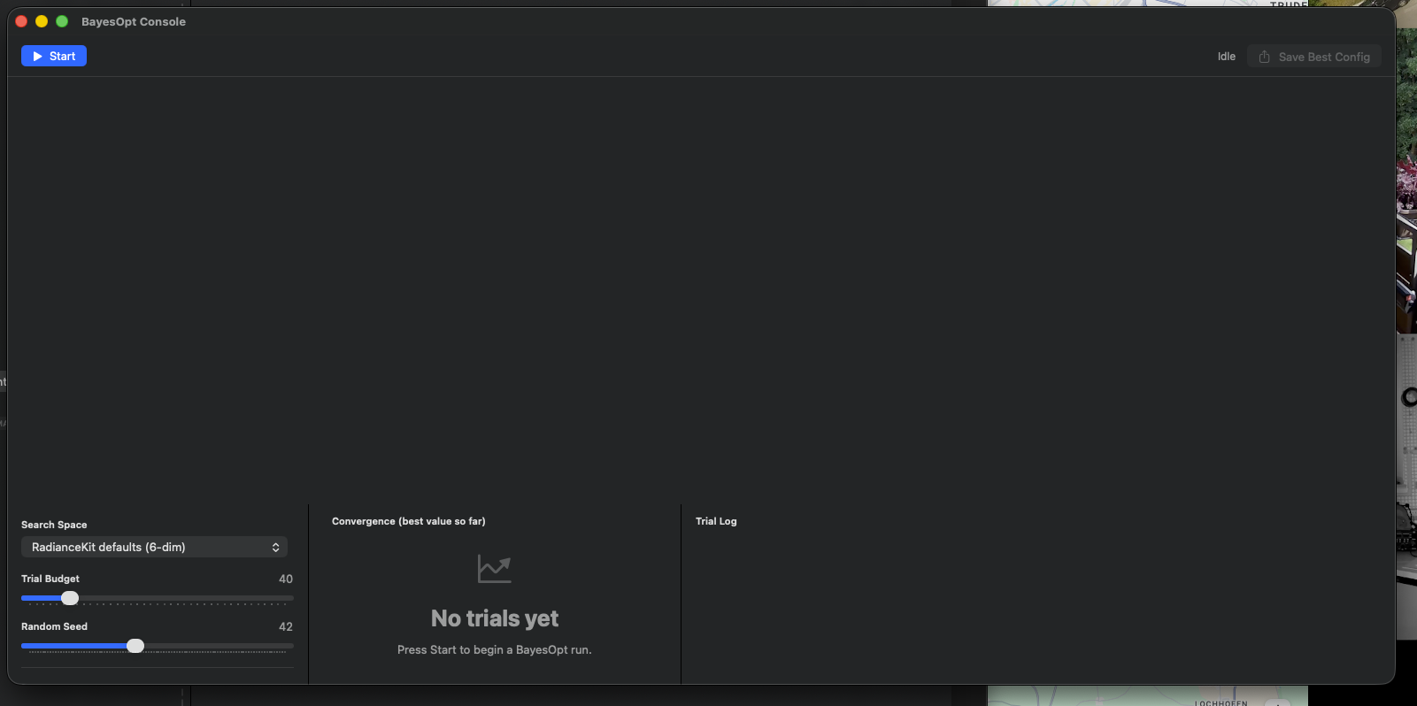
Empty state with search-space picker (RadianceKit defaults (6-dim)), trial-budget slider (default 40), random seed (42), and three empty panels for the convergence chart, trial log, and search-space parameter list. The convergence chart and trial table fill in once a run has been started — see the next figure.
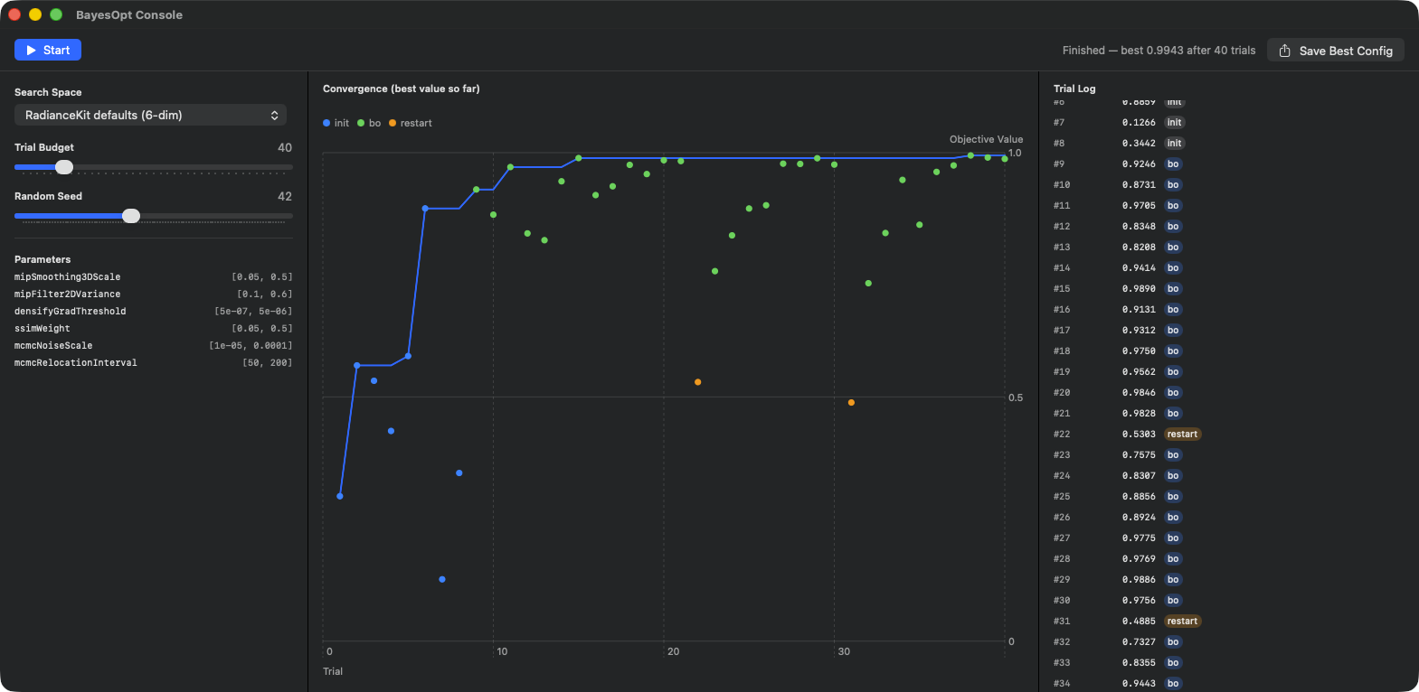
Status top right "Finished — best 0.9943 after 40 trials", next to it the "Save Best Config" button; top left the "Start" button. Left sidebar: search-space picker set to RadianceKit defaults (6-dim), trial budget 40, random seed 42. The parameter list shows the six hyperparameters to tune, with their value ranges: mipSmoothing3DScale [0.05, 0.5], mipFilter2DVariance [0.1, 0.6], densifyGradThreshold [5e-07, 5e-06], ssimWeight [0.05, 0.5], mcmcNoiseScale [1e-05, 0.0001], mcmcRelocationInterval [50, 200]. Center: convergence chart "Convergence (best value so far)" (X = trial index 0–40, Y = objective value 0–1) — blue points = initial samples, green points = BayesOpt acquisition, orange points = restart trials (#22 with 0.5303 and #31 with 0.4885). The blue best-value line rises steeply until trial ~5, then only marginal improvement until trial ~13, after which there's a flat plateau near 1.0. Right sidebar: trial log, here scrolled to trials #8–#36, with score + tag (init/bo/restart). The Save Best Config button top right writes bayesopt-best.json.
What it is: A Bayesian optimization console for hyperparameter search. Bayes-opt is an automatic procedure that tries to find the optimal point of an unknown function using as few experiments as possible — typically: "which combination of Gaussian upper bound, SSIM weight, and densify threshold delivers the best PSNR for my scene class?" Instead of a grid of 6^4 = 1296 trials, Bayes-opt tries around 40–100 informed trials and gets close to the optimum that way.
Important: The version currently shipped in the app does not run the optimization against real training runs (that would take days), but against a synthetic demo objective — a multi-modal landscape with hill-climbing character plus slight noise. This is intentional: the window is meant to show you the optimizer's behavior (convergence progression, sample points, best-so-far) and let you understand the search-space definitions. For real training-driven BayesOpt runs (as were performed while developing the bundled presets), a separate evaluation path outside the app is used; this window is the live variant for watching along.
Three use cases: 1. You want to understand how BayesOpt works — then start a demo run and watch the convergence chart. 2. You're planning a new scene class (say, "aquariums" or "antique furniture") for which the fifteen built-in presets don't fit perfectly. Mentally define a search space, test it here with "Bowl demo (1-dim)" or "densify-until + ssim-weight + grad-thresh", then export the best config as JSON and use it as a starting point for a real training run. 3. You want to inspect the built-in default search spaces (Mip subset, RadianceKit Defaults) — these are listed in the parameter panel of the left sidebar.
- Convergence chart (center column): Y = best objective function value achieved so far. X = trial index. Initially rises steeply (BayesOpt tries the initial samples randomly, some of them get lucky), then increasingly flattens out because the near-optimum region has been exhausted. If the line stays flat for 20+ trials, you can stop the run — further trials won't gain anything more. The individual points in the chart are the individual trial values (i.e. not "best so far"), colored by phase: blue = initial sample, green = bayesopt acquisition, orange = restart. - Trial table (right column): #1, #2, #3, … each with value and phase tag. The best trial so far is marked with a yellow star. From the table you can identify the best trial and look at its parameter values later during export. - Search-space inspector (left sidebar): shows, for the selected preset, all parameter names and their search ranges [lo, hi]. If you're on the "RadianceKit defaults (6-dim)" preset, you'll see e.g. "densifyGradThreshold [5e-7, 5e-6]" — i.e. log-uniform between these two values.
Select preset "RadianceKit defaults (6-dim)", trial budget 40, seed 42. Click "Start". Watch: the first 8 trials are blue (initial samples, Latin hypercube), the following ones green (BayesOpt-acquired). The convergence chart rises steeply until trial ~13, after which it flattens out. Around trial ~30–40 the best value stabilizes. Click "Save Best Config" — a bayesopt-best.json is saved with the preset name, trial index, value, and the decoded parameter values. You can then manually adopt this JSON into your preset definition.
W30Button "Start"
WHERE
Toolbar left, in the idle/finished state.
TECHNICAL
Resets the trial list, switches into the running state, generates a new run ID (for stale detection with multiple start clicks) and creates a fresh pause gate. Then it starts a background task that runs the optimizer as an asynchronous stream. The number of initial samples grows with the budget, but at most up to 8 — so typically 8 Latin-hypercube samples from a budget of 28 upward, fewer with a smaller budget. Trial updates are received incrementally and appended to the list. Stale-run protection: if a second start click sets a new run ID in the meantime, updates from the old run are discarded.
Primary-action style for the prominent button look.
W31Button "Pause"
WHERE
Toolbar left, in the running state.
TECHNICAL
Activates the pause gate and switches into the paused state. The actual effect: the runner waits in a 50 ms polling loop before evaluating the next objective function. This means a trial currently running is completed (it's synthetic and only takes microseconds), but no further trial is triggered. Once resume runs, it picks up where it left off.
W32Button "Stop"
WHERE
Toolbar left, in the running and paused states.
TECHNICAL
Cancels the runner task, nulls the reference, releases the pause gate (if it was still paused), and switches into the finished state (if trials exist) or the idle state (if none exist). The trials already computed remain visible in the list — Stop doesn't delete them. Destructive button role shows the button in red, because it aborts the run.
W33Button "Resume"
WHERE
Toolbar left, in the paused state.
TECHNICAL
Releases the pause gate and switches back into the running state. The runner task is already running (it's waiting in the polling loop); as soon as the loop notices that the pause has been lifted, it continues and starts the next trial.
W34Button "Save Best Config"
WHERE
Toolbar right, always visible (but grayed out as long as no best run exists yet).
TECHNICAL
Opens a save dialog with the default filename bayesopt-best.json, restricted to JSON. After confirmation, a payload dictionary is built: preset name, trial index, value (objective score), parameters (dictionary of decoded parameter names → values). The decoding projects the normalized search-space coordinates in [0,1]^d back into the original value range (with log-uniform/linear/integer scales as appropriate). The JSON output is pretty-printed and with sorted keys. On a write error, the current demo version silently ignores it — no error UI, because this is a demo path.
The button remains gray as long as no trial has run.
W35Picker "Search Space" preset
WHERE
Left sidebar, top.
TECHNICAL
Menu picker with four preset options: - "RadianceKit defaults (6-dim)" — the full default search space with all six standard hyperparameters. - "Mip subset (2-dim)" — only mipSmoothing3DScale [0.05, 0.5] log-uniform and mipFilter2DVariance [0.1, 0.6] linear. Useful if you want to tune mip splatting for a scene class. - "densify-until + ssim-weight + grad-thresh" — three densify-relevant parameters (densifyGradThreshold log-uniform, ssimWeight linear, densifyUntilIter integer). - "Bowl demo (1-dim)" — pedagogical single-parameter search space for "how BayesOpt works" demos.
While a run is active, the search space cannot be switched (this would confuse the optimizer).
W36Slider "Trial Budget"
WHERE
Left sidebar, below the search-space picker.
TECHNICAL
Slider from 10 to 200, step size 5. Default 40. This means: BayesOpt may make at most N trials. Of these, the first few are initial samples (Latin hypercube), the rest are real BayesOpt trials. Rules of thumb for practice: a search space with d dimensions needs roughly ten to twenty times d in trials for a good optimum. So for 6-dim defaults, 60–120; for 2-dim Mip subset, 20–40; for 1-dim Bowl demo, 10–20.
The slider is disabled during the run.
W37Slider "Random Seed"
WHERE
Left sidebar, below the budget slider.
TECHNICAL
Slider from 1 to 100, step size 1. Default 42. The seed is passed both to the initial Latin-hypercube samples and to the noise component of the demo objective. Reproducibility: the same seed + same search space + same budget produces an exactly identical trial sequence. Useful for "do all your colleagues get the same run when they rebuild the demo?". Disabled during the run.
W38Chart (Convergence)
WHERE
Center column of the window.
TECHNICAL
Swift Charts diagram with two layers: 1. a line for "best-value-so-far" per trial — a monotonically rising or level curve in accent color. 2. a point per trial with the individual objective value, colored by phase. Symbol size 40. Three phase labels: "init" (blue), "bo" (green), "restart" (orange).
A small legend shows the phase colors top left. If the trial list is empty (before the first start), an empty- state display with a chart icon and hint "Press Start to begin a BayesOpt run." is shown instead.
W39Table (Trial Log)
WHERE
Right column of the window.
TECHNICAL
Scroll area with lazily stacked trial rows. Per row a horizontal stack: trial number (3-digit monospaced, left), value (monospaced, right-aligned, 70 pt wide), phase tag (capsule, filled at 25% opacity — gray for "init", blue for "bo", orange for "restart"; these are deliberately different colors than the point colors in the chart next to it), optionally a yellow star if this trial is currently the best. An auto-scroll mechanism jumps automatically to the end as soon as a new trial is added — so you can follow along the live progression at the bottom of the screen without scrolling yourself.
Main Window: Loss History and Gaussian Count (I39–I41, Cross-Reference)
Three of the Inspector displays in the main window deserve their own explanation, because they are visible constantly during a running training run and because there are important rules of thumb for when the curve looks healthy. The displays sit in the Inspector in the Progress section, in the expandable group Loss History (see chapter 2 — Inspector), and complement the holdout analysis from the Aux window above.
When is the loss curve healthy? A healthy loss curve shows three phases: (1) Warmup — during the first 200–500 iterations, the loss drops steeply from high (typically 0.15–0.25 for combined L1+SSIM, depending on the scene) to roughly half that. If the loss does NOT drop in this phase, the input is usually wrong (broken images, bad SfM poses, too few initial Gaussians). (2) Densification — between ~500 and densifyUntilIteration (classic 15K, MCMC up to 20K or 25K), the loss keeps falling, often with small downward jumps when densify operations insert new Gaussians and the optimizer makes use of them. The Gaussian count rises during this phase. (3) Refinement — after that, the loss runs into a flattening tail. Typical final values for orientation: a well-lit object scene (such as Tanks-&-Temples Truck with P4 Quality) lands at L1 ≈ 0.023, while expansive outdoor scenes like those from Mip-NeRF 360 naturally stay above that (0.04–0.07).
What does a plateau mean? A plateau (the loss curve runs horizontally over several thousand iterations) has two interpretations: (a) the model has converged, further training won't achieve anything more — that's the good case. (b) the model is stuck (local minimum, poor gradient information, a cap at the buffer limit) — the bad case. Both look identical on the chart. To tell them apart: look at the Gaussian count. If it's also flat AND close to the MCMC cap (e.g. 150K of 150K with the preset P8 Quality (MCMC)), you're at the limit — either raise the cap or accept the plateau. If the Gaussian count is still growing but the loss isn't dropping, that's stuck.
When to stop vs. keep training? Rule of thumb: 10K iterations with no improvement in the min loss → stop, further iterations are wasted. Before that: via the Training menu → Continue Training → "+5,000 iterations" you can still append an extension if you're seeing marginal improvement (there's no keyboard shortcut for this). Note: with MCMC, the plateau is often genuine — the cap is the natural limit.
A Gaussian count plateau is NOT a "done" signal. It only means that MCMC has reached its cap or that Classic Densification has been exhausted. The real "done" question is only answered by PSNR/SSIM/LPIPS on an independent test set — the numbers for that are in the benchmark reports you evaluate in the Pareto Dashboard (W13–W22). The Holdout window (W23–W29) does not provide these metrics; it only judges whether your camera set allows for a fair split into training and test viewpoints in the first place.
PSNR/holdout is the truth, loss is just a proxy. The loss is a relative metric: it drops as your model adapts to the training views. A low loss, however, doesn't automatically mean a good model — if the model has memorized the training images (overfitting), the loss would be small, but the PSNR on unseen views (holdout) would be poor. Therefore: for the final quality assessment, always look at the holdout metrics, not at the end loss alone.
Rule-of-Thumb Box
- User Guide and Keyboard Shortcuts are static help — fast for keyword questions, use this manual for depth. - Open Manage Storage as soon as the disk drops below 10% free space. Logs and imports staging are the usual culprits. - Pareto Dashboard only makes sense after at least three or four training reports. X-axis = cost (Time / Gs), Y-axis = quality (PSNR / SSIM). The Pareto front shows the efficient combinations. - Use Holdout Analysis before publishing PSNR benchmarks with others — it ensures your test set is truly representative. The exported fold split is for external tools; RadianceKit keeps training against "every-8th". - BayesOpt Console is primarily a learning and inspection tool for search-space definitions — it computes against a demo function, not against real training runs. - Loss plateau and Gaussian-count plateau must be interpreted separately. Cap limit is not a "done" signal. Real quality is only measured by holdout PSNR. - 10K iterations without min-loss improvement → stop training.